Pre-processing

For pre-processing, like flat correction and phase retrieval, there are the commands tofu flatcorrect, tofu preprocess, tofu find-large-spots and tofu sinos. Please refer to tofu command --help for a list of complete parameters, many of the commands below share a lot of them, e.g. --darks are available in almost all of the commands.

Flatcorrect

You can use command tofu flatcorrect to flat correct projections. For doing this, you need a set of dark fields (images), flat fields and projections. It is good to have many dark and flat fields to reduce noise. The command computes an “average” dark and flat field based on the reduction mode below and then computes the corrected projections. The most important arguments are:

--projections: Location with projections (default: None);
--darks: Location with darks (default: None);
--flats: Location with flats (default: None);
--reduction-mode: controls the computation of dark field and flat field, one of: Average or Median;
--fix-nan-and-inf: suppress NaN (not a number) and infinite numbers which may be caused by zero division ;
--absorptivity: compute $log (I_0 / I)$ , where $I_0$ is the flat field and $I$ is the projection. If you do not specifiy this option, the result is simply $I / I_0$ ;
--dark-scale: multiplies the dark field with this value;
--flat-scale: multiplies the flat field with this value (e.g. you need to reduce exposure time by half in order not to saturate, then you would set this to 2);
--flats2: this argument is useful when you have two sets of flat fields, one before the projection acquisition and one after. The flat field for current projection in the sequence is linearly interpolated from the averate first and second flat field.

Preprocess

tofu preprocess is a command capable of:

flat correction;
applying cone beam weight;
phase retrieval;
projection filtering for back projection.

You may use the arguments in Flatcorrect to set up the flat correction part of the command, --transpose-input transposes the images.

Cone Beam Weight

Cone beam weight coordinates are defined as follows:

x = lateral dimension;
y = beam propagation dimension;
z = vertical dimension;

and the following arguments apply:

--source-position-y: Y source position (along beam direction) in multiples of nominal detector pixel size;
--detector-position-y: Y detector position (along beam direction) in multiples of nominal detector pixel size;
--center-position-x: X rotation axis position on a projection in pixels;
--center-position-z: Z rotation axis position on a projection in pixels;
--axis-angle-x: Rotation axis rotation around the x axis (laminographic angle, 0 = tomography) in degrees.

Phase retrieval

Phase retrieval converts the interference pattern from propagation-based phase contrast to the actual phase or even projected thickness, depending on the algorithm used and arguments. It is turned on if --energy and --propagation-distance arguments are specified. The algorithms are:

tie: Transport of Intensity Equation;
ctf: Contrast Transfer Function;
qp: Quasiparticle Approach;
qp2: modified Quasiparticle approach where frequencies are not suppressed by zero but a small constant with the sign of the CTF sign.

The arguments are:

--retrieval-method: Phase retrieval method, one of [tie, ctf, qp, qp2] (default: tie);
--energy: X-ray energy [keV] (default: None, meaning: turn phase retrieval off);
--propagation-distance: Sample <-> detector distance (if one value, then use the same for x and y direction, otherwise first specifies x and second y direction) [m] (default: None, meaning: turn phase retrieval off);
--pixel-size: Pixel size [m] (default: 1e-06);
--regularization-rate: Regularization rate (the value of $log_{10} (\delta / \beta)$ , where $\delta$ is the real part of the complex refractive index and $\beta$ the imaginary; typical values between [2, 3]) (default: 2);
--delta: Real part of the complex refractive index of the material. If specified, phase retrieval returns projected thickness, if not, it returns phase (default: None);
--retrieval-padded-width: Padded width used for phase retrieval (default: 0, meaning: automatic);
--retrieval-padded-height: Padded height used for phase retrieval (default: 0, meaning: automatic);
--retrieval-padding-mode: Padded values assignment, one of [none, clamp, clamp_to_edge, repeat, mirrored_repeat] (default: clamp_to_edge) (refer to <addressing mode> section in the OpenCL documentation for more information);
--thresholding-rate: Thresholding rate (typical values between [0.01, 0.1]) (default: 0.01);
--frequency-cutoff: Phase retrieval frequency cutoff [rad] (default: 1e+30);

Projection Filtering for Back Projection

Projection filtering is done prior to the back projection step. In case you need to perform many 3D reconstructions by filtered back projection on the same data set, you might want to apply the filter before the back projections. The arguments are:

--projection-filter: Projection filter, one of [none, ramp, ramp-fromreal, butterworth, faris-byer, bh3, hamming] (default: ramp-fromreal);
--projection-filter-cutoff: Relative cutoff frequency (default: 0.5);
--projection-padding-mode: Padded values assignment, one of [none, clamp, clamp_to_edge, repeat, mirrored_repeat] (default: clamp_to_edge) (refer to <addressing mode> section in the OpenCL documentation for more information);

Generating Sinograms

tofu sinos is needed when you want to remove rings from your reconstructed slices (which manifest as stripes in sinograms). After this, you can use tofu tomo for the 3D reconstruction. Arguments:

--pass-size: Number of sinograms to process per pass, which is useful if your PC has little memory (CPU RAM, sinogram generation does not take place on GPUs) (default: 0, meaning: automatic);
--y: Vertical coordinate from where to start reading the input image: controls detector row of the first sinogram (default: 0);
--height: Number of rows which will be read: controls number of sinograms (default: None, meaning: all).

You may also perform flat correction in one step by using the flat correction arguments. For a full list, see tofu sinos --help.

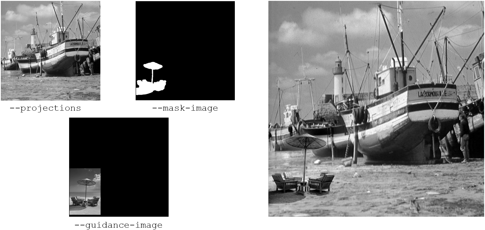
Inpainting

Inpainting is useful when we need to (a) seamlessly blend a part of one image into another, or (b) if we want to interpolate some corrupted region in an image. In the context of 3D reconstruction, inpainting can be used in Removing Broad Rings from Tomographic Slices. The algorithm is based on the Fourier transform method in [Morel et al., 2012].

Seamless Cloning

One may seamlessly blend two images like this:

tofu inpaint --guidance-image guidance.tif --projections boat.tif --mask-image mask.tif --preserve-mean --output inpainted.tif

Which will produce the following output:

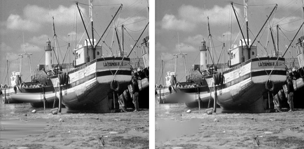
Interpolation of a corrupted region requires the same command, just without the specification of the guidance image:

tofu inpaint --projections boat.tif --mask-image mask.tif --preserve-mean --output inpainted.tif

# For comparison: horizontal-interpolate
ufo-launch [read path=boat.tif, read path=mask.tif] ! horizontal-interpolate ! write filename=horiz-interpolate.tif

Side-by-side comparison of the result of horizontal-interpolate (left) and inpainting (right) generated with the above commands:

Harmonization of Image Borders (for the Removal of the Power Spectrum Cross)

Discrete Fourier transform assumes that images are N-periodic, i.e. after pixel N-1, pixel 0 comes again and so on. The transitions between image borders thus often contain harsh discontinuities which are reflected in the Fourier transform and manifest as a cross in the power spectrum aligned with the coordinate axes and crossing the (0, 0) frequency. We can remedy this by blending the opposing borders.

In the image below (boat cropped to 371 x 371 pixels), on the left is the original image after swapping quadrants to emphasize the border discontinuities. In the middle is the harmonized image without padding of the Fourier transform and on the right with padding from the original 371 x 371 to 512 x 512 pixels. Commands used for their generation are shown below (with the additional swapping of quadrants).

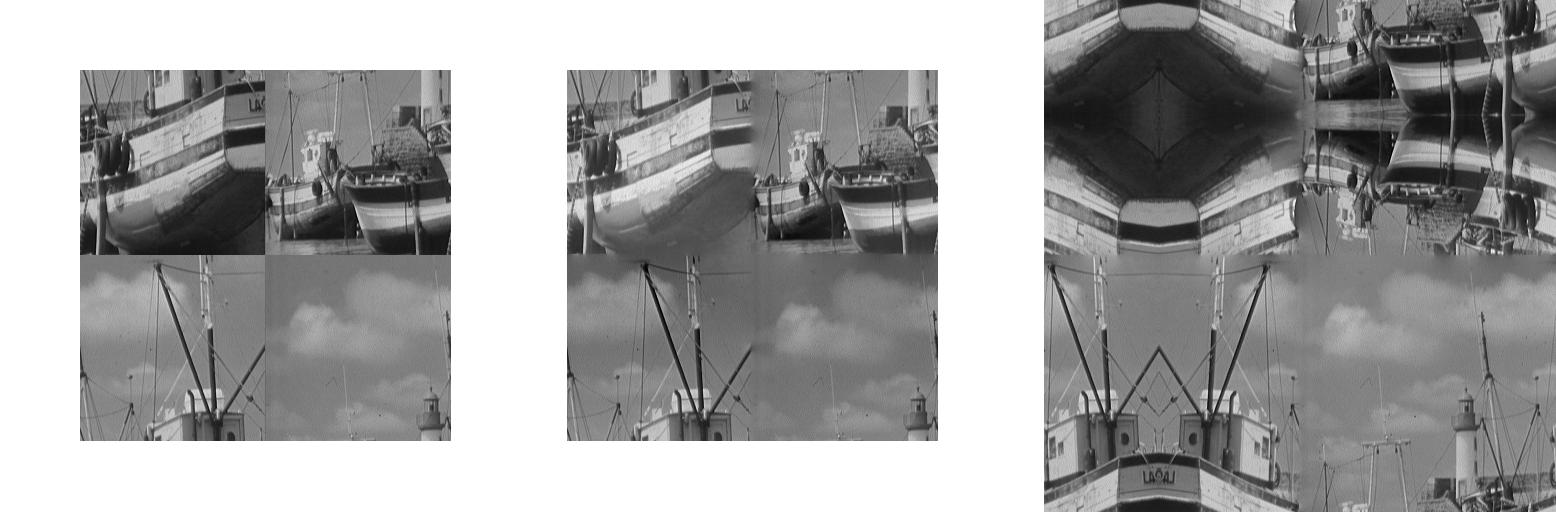
Image before and after border harmonization

tofu inpaint --projections input.tif --preserve-mean --harmonize-borders --output middle-harmonized.tif
tofu inpaint --projections input.tif --inpaint-padded-width 512 --inpaint-padded-height 512 --inpaint-padding-mode mirrored_repeat
--preserve-mean --harmonize-borders --output right-harmonized.tif

Below are the power spectra of the respective images above and below the commands to generate them. Note the cross in the left image and how the positive and negative frequencies are starting to get mixed in the right one, which is caused by mirrored_repeat padding mode.

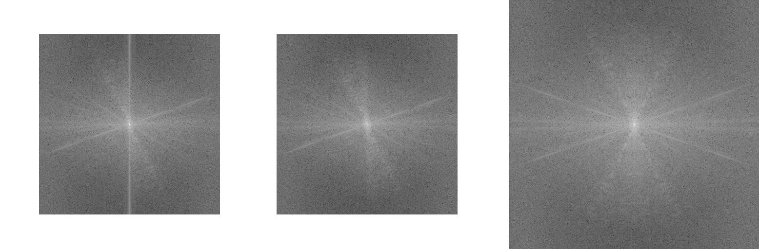
Power spectra of an image before and after border harmonization

ufo-launch read path=input.tif ! fft dimensions=2 ! power-spectrum ! calculate expression="'log(v)'" ! swap-quadrants
    ! write filename=left-power-spectrum.tif
ufo-launch read path=middle-harmonized.tif ! fft dimensions=2 ! power-spectrum ! calculate expression="'log(v)'"
    ! swap-quadrants ! write filename=middle-power-spectrum.tif
ufo-launch read path=right-harmonized.tif ! fft dimensions=2 !  power-spectrum ! calculate expression="'log(v)'"
    ! swap-quadrants ! write filename=right-power-spectrum.tif

Removing Broad Rings from Tomographic Slices

tofu find-large-spots finds large scintillator spots of extreme intensity (zero or maximum) on projections. These spots cannot be flat corrected and cause broad ring artifacts in the reconstructed tomographic slices (see Removing Narrow Rings from Tomographic Slices for filtering narrow rings). By finding and suppressing these spots prior to 3D reconstruction, one can obtain much cleaner slices.

The algorithm creates a mask which you can then use to filter the erroneous regions. It works on flat fields, first, it removes the low frequency components of a flat field, then thresholds it and from the found extreme intensities “grows” until another threshold is hit. The arguments are:

--images: Location with input images (default: None);
--gauss-sigma: Gaussian sigma for removing low frequencies (filter will be 1 - gauss window) (default: 0.0, meaning: turn low-frequency removal off);
--blurred-output: Path where to store the blurred input (default: None);
--spot-threshold: Pixels with grey value larger than this are considered as spots (default: 0.0);
--spot-threshold-mode: Pixels must be either “below”, “above” the spot threshold, or their “absolute” value can be compared, one of [‘below’, ‘above’, ‘absolute’] (default: absolute);
--grow-threshold: Spot growing threshold, if 0 it will be set to FWTM times noise standard deviation (default: 0.0, meaning: automatic);
--find-large-spots-padding-mode: Padded values assignment for the filtered input image, one of [none, clamp, clamp_to_edge, repeat, mirrored_repeat] (default: repeat) (refer to <addressing mode> section in the OpenCL documentation for more information).

Broad ring filtering example:

# Flat correction
tofu flatcorrect --projections projections/ --darks darks/ --flats flats/ --fix-nan-and-inf --output fc.tif
--output-bytes-per-file 1t

# Finding the spots
tofu find-large-spots --output-bytes-per-file 0 --number 1 --output mask.tif --spot-threshold 500.0 --find-large-spots-padding-mode repeat
--spot-threshold-mode absolute --gauss-sigma 10.0 --images flats/

# Filtering the spots by horizontal linear interpolation
ufo-launch -q [read path=fc.tif, read path=mask.tif] !  horizontal-interpolate ! write filename=interpolated.tif
bytes-per-file=1000000000000 tiff-bigtiff=True

# Or by inpainting
tofu inpaint --projections fc.tif --mask-image mask.tif --preserve-mean --output interpolated.tif

Removing Narrow Rings from Tomographic Slices

This is achieved by removing stripes in sinograms which translate to half-rings after 3D reconstruction. This algorithm is most suitable for narrow ring artifacts as opposed to the Removing Broad Rings from Tomographic Slices.

In the following example we assume sinogram width 2016 pixels and height 3000 pixels. In order to suppress convolution artifacts, we pad the sinogram by a factor of 2 in every dimension and then need to manually compute the next power of two required by UFO’s fft filter. Moreover, we place the original sinogram in the middle of the padded one and use the mirrored_repeat approach to fill the padding pixels with data instead of just using zeros. The computation is 2 x 2016 = 4032 and the next power of two is 4096, 2 x 3000 = 6000 with the next power of two 8192. We want to place the sinogram in the middle, so starting x is (4096 - 2016) / 2 = 1040 and starting y is (8192 - 3000) / 2 = 2596.

Put together on the command line, we arrive at the narrow ring filtering example:

# Create sinograms
tofu sinos --number 3000 --projections interpolated.tif --output sinos.tif --output-bytes-per-file 1t

# Filter narrow stripes in sinograms in frequency space
ufo-launch -q read path=sinos.tif ! pad width=4096 height=8192 x=1040 y=2596 addressing-mode=mirrored_repeat !
fft dimensions=2 ! filter-stripes horizontal-sigma=100.0 vertical-sigma=2.0 ! ifft dimensions=2 !
crop width=2016 height=3000 x=1040 y=2596 ! write filename=filtered-sino.tif bytes-per-file=1000000000000
tiff-bigtiff=True

Note

We do our best to keep the argument names consistent with the parameters from UFO Framework but sometimes that would lead to ambiguities and the arguments in tofu are prefixed with the filter name, like --output-bytes-per-file.

Also, high-level features like using k, m, g, t with --output-bytes-per-file is a feature of tofu and is not included in the low-level ufo-launch command.